The Geography of Generosity
A regression analysis of neighborhood socioeconomics and taxi tipping behavior in Chicago.
Abstract
This report presents a comprehensive regression analysis of the factors influencing taxi tipping behavior in Chicago, specifically isolating the impact of neighborhood socioeconomic status on driver compensation. While tipping constitutes a critical portion of service worker income, the specific drivers of generosity, beyond the cost of the service itself, remain largely opaque. Utilizing a massive public dataset of Chicago Taxi Trips spanning a decade (2013–2023) merged with socioeconomic data from the American Community Survey (ACS), this study investigates whether a measurable "geography of generosity" exists within the city.
The methodology employed rigorous data preprocessing, including the removal of outliers and the feature engineering of an Estimated Mean Income variable derived from binned census counts. To satisfy the assumptions of linear regression, the highly right-skewed target variable (Tip Percentage) was log-transformed. A Multiple Linear Regression (MLR) model was constructed to test the central hypothesis, controlling for significant confounding variables such as trip fare, trip duration, day of the week, and hour of the day. Model validity was confirmed through Variance Inflation Factor (VIF) testing to rule out multicollinearity and an 80/20 train-test split validation, which yielded a Root Mean Squared Error (RMSE) of 1.61.
The analysis confirms a statistically significant positive relationship (p < 2.2e-16) between a neighborhood's estimated mean income and the average tip percentage, holding all other factors constant. Furthermore, a residual analysis was conducted to calculate a "generosity score" for each of Chicago's 77 community areas, identifying neighborhoods that consistently tip above or below the model's predictions. These findings provide data-driven evidence that geography and local economic conditions are significant, independent predictors of economic behavior in the transportation sector.
Introduction
Background
Tipping is one of the most pervasive yet poorly understood economic behaviors in the United States. Unlike fixed pricing models where labor costs are embedded in the service fee, the taxi and transportation industry relies heavily on a system of voluntary subsidization. For the thousands of taxi drivers operating in metropolitan areas like Chicago, tips are not merely a bonus for exceptional service; they constitute a critical, often volatile, component of their total livelihood.
In the modern "gig economy," uncertainty is the norm. A driver's income fluctuates based on traffic, weather, and competition from ride-sharing platforms. However, one variable remains particularly opaque: the generosity of the passenger. While social norms dictate a standard tipping range (typically 15–20%), individual adherence to this norm varies wildly. Is this variation purely random, driven by the mood of the passenger? Or are there deeper, structural predictors of generosity rooted in the socioeconomic fabric of the city itself? Understanding these patterns is not just an academic exercise; for a driver making strategic decisions about where to operate, it is a matter of economic efficiency.
Problem Statement
While anecdotal evidence among drivers suggests that certain neighborhoods are "better" for tips than others, this wisdom is often clouded by confounding variables. A trip from a wealthy neighborhood might yield a higher absolute tip simply because the destination is further away (resulting in a higher fare), not because the passenger is inherently more generous.
This study seeks to disentangle these factors. By merging ten years of trip data from the City of Chicago's Taxi Trips dataset with socioeconomic data from the American Community Survey (ACS), we aim to isolate the specific impact of neighborhood wealth on tipping behavior. The core problem this report addresses is whether a "geography of generosity" exists — a measurable, statistically significant pattern where the socioeconomic status of a pickup location predicts the percentage a passenger is willing to tip, independent of the trip's cost, duration, or timing.
Research Questions
To investigate this phenomenon, this report addresses four specific research questions:
- Q1: Is there a statistically significant relationship between the estimated mean income of a Chicago community area and the tip percentages given on taxi trips originating from that area?
- Q2: Does this relationship hold true even after controlling for confounding variables such as the trip fare amount, trip duration, time of day, and day of the week?
- Q3: Can we quantify the "price of generosity"? Specifically, for every unit increase in a neighborhood's mean household income, what is the expected percentage increase in the tip?
- Q4: Which specific Chicago neighborhoods exhibit the highest and lowest levels of "generosity" (tipping above or below the expected model prediction)?
Central Hypothesis
Based on the economic theory that disposable income correlates with discretionary spending, we propose the following central hypothesis:
Hypothesis (H₁): Taxi trips originating from community areas with higher socioeconomic status (measured by estimated mean household income) will exhibit a higher average tip percentage compared to trips from lower-income areas, even when controlling for trip length, fare, and temporal factors.
Conversely, the Null Hypothesis (H₀) posits that once the mechanics of the trip (fare and duration) are accounted for, the socioeconomic status of the pickup location has no statistically significant effect on the tip percentage.
Report Structure
The remainder of this report is organized as follows:
- Data & Methodology details the acquisition, cleaning, and merging of the Chicago Taxi and ACS datasets, including the feature engineering required to calculate neighborhood income estimates.
- Exploratory Data Analysis presents a visual investigation of the variables, identifying key trends and potential modeling pitfalls such as multicollinearity.
- Regression Modeling & Results documents the step-by-step construction of the regression models, diagnostic testing, and validation procedures.
- Analysis & Interpretation synthesizes the findings to answer the research questions and presents the final "Geography of Generosity" rankings.
- Conclusion summarizes the study's implications and limitations.
Data & Methodology
To analyze the relationship between neighborhood socioeconomic status and tipping behavior, a robust data pipeline was constructed to integrate transportation records with census-level demographic data. This section details the data acquisition, cleaning, feature engineering, and transformation processes employed in the study.
Data Sources
This analysis relies on the synthesis of three distinct public datasets provided by the City of Chicago Data Portal. The table below summarizes the sources utilized.
| Dataset Name | Source Description | Key Variables Utilized |
|---|---|---|
| Chicago Taxi Trips | A comprehensive log of taxi trips reported to the City of Chicago from 2013 to 2023. | Trip Start Timestamp, Trip Seconds, Trip Miles, Fare, Tips, Pickup Community Area |
| Census Data – Selected Socioeconomic Indicators | American Community Survey (ACS) 5-Year Estimates for Chicago community areas. | Community Area Name, Household Income Bins (e.g., "Under 25k–$50k") |
| Boundaries – Community Areas | A GIS-based lookup table defining the names and numeric identifiers of Chicago's 77 community areas. | AREA_NUMBE (ID), COMMUNITY (Name) |
Data Acquisition and Integration
A primary challenge in merging these datasets was a schema mismatch between the transportation and census data. The Taxi Trips dataset identifies pickup locations using a numeric identifier (e.g., 8 for Near North Side), while the ACS census data utilizes string labels (e.g., "NEAR NORTH SIDE").
To resolve this, the Boundaries dataset served as a bridge table. A three-stage join process was executed:
- Standardization. All community names in the lookup table and ACS data were converted to uppercase to ensure string matching consistency.
- Intermediate Join. The ACS socioeconomic data was joined with the Boundaries lookup table to append the correct numeric ID (
community_num_key) to each neighborhood's profile. - Final Merge. The enhanced ACS data was left joined to the primary Taxi Trips dataset on the Pickup Community Area key, effectively stamping every taxi trip with the socioeconomic profile of its origin neighborhood.
Data Cleaning and Preprocessing
Raw data from the City of Chicago portal contains formatting inconsistencies and entry errors that required significant cleaning before analysis.
- Sanitization of Currency. Columns such as Fare and Tips were originally stored as character strings containing "$" symbols. These were stripped of non-numeric characters and converted to double precision floating point numbers.
- Filtering Invalid Records. To ensure economic viability, the dataset was filtered to exclude impossible or non-commercial trips. Records were removed if:
Fare <= 0(System errors or voided trips)Tips < 0(Chargebacks or errors)Trip Seconds <= 0(Instantaneous timestamps implying system errors)
- Missing Values. Trips with missing Pickup Community Area data or those that could not be joined to a valid census tract were excluded, as they could not contribute to the geospatial analysis.
Feature Engineering
Feature engineering was critical to transforming raw administrative logs into meaningful predictors for regression modeling.
The Target Variable: Tip Percentage
The raw Tips column is an absolute value, which naturally scales with the fare. To measure generosity rather than cost, a new target variable was calculated:
The Socioeconomic Predictor: Estimated Mean Income
The provided ACS dataset did not contain a pre-calculated Mean Household Income or Median Household Income. Instead, it provided binned frequency counts of households (e.g., number of families earning between 49,999).
To create a continuous quantitative predictor, a weighted arithmetic mean was engineered for each community area. We assigned a midpoint value to each income bin and calculated the Estimated Mean Income as follows:
The assumed midpoints were:
| Income Bin | Midpoint |
|---|---|
| Under $25,000 | $12,500 |
| 49,999 | $37,500 |
| 74,999 | $62,500 |
| 125,000 | $100,000 |
| $125,000+ | $150,000 (conservative estimate for the open-ended upper bin) |
Time-Based Covariates
Tipping behavior is hypothesized to vary by time of day and day of the week. Using the lubridate package, the Trip Start Timestamp was parsed to extract:
Trip_Hour(0–23)Trip_Day_Of_Week(Mon–Sun)Trip_MonthandTrip_Year(to control for seasonality and inflation)
Variable Transformation for Modeling
Linear regression relies on assumptions of normality and homoscedasticity. Initial exploratory analysis revealed significant violations of these assumptions, necessitating transformation.
Handling Outliers
The Tip_Percentage variable contained extreme outliers (e.g., 1000%+ tips likely due to data entry errors). To prevent these from skewing the model, the variable was capped at the 99th percentile.
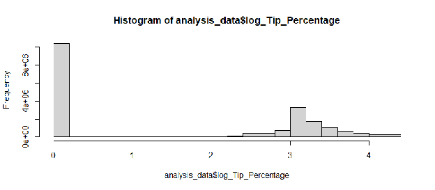
Log-Transformation of the Target
As shown in Figure 1.1, the distribution of tip percentages was highly right-skewed, with a massive concentration at 0% and a long tail. This violates the normality assumption of Ordinary Least Squares (OLS) regression.
To correct this, a log-transformation was applied:
Note: A constant of 1 was added to handle cases where the tip was 0%, as ln(0) is undefined.
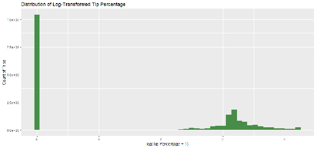
As illustrated in Figure 1.2, this transformation successfully normalized the distribution, producing a bell-shaped curve suitable for linear modeling.
Factorization
Qualitative variables such as Trip_Day_Of_Week and Trip_Hour were explicitly converted to unordered factors. This ensures the regression model treats them as distinct categories (creating dummy variables) rather than continuous numeric values (which would incorrectly imply that 11:00 PM is "greater than" 10:00 PM).
Software and Performance Optimization
The analysis was conducted using R Studio. Due to the magnitude of the dataset (millions of rows), the data.table package was utilized for high-performance memory management and aggregation during the modeling phase, while the tidyverse suite (dplyr, ggplot2, readr) was employed for initial data manipulation and visualization.
Exploratory Data Analysis
Before constructing formal regression models, a comprehensive Exploratory Data Analysis (EDA) was conducted to visualize the underlying structure of the dataset, validate assumptions, and detect potential anomalies. This phase served two primary purposes: (1) to assess the visual validity of the central hypothesis linking neighborhood income to tipping behavior, and (2) to identify confounding variables and multicollinearity that could destabilize the final model.
Univariate Analysis
The primary target variable, Tip_Percentage, exhibited extreme right skewness. However, the distribution of the key predictor, Estimated_Mean_Income, also warranted examination to understand the economic diversity of the sample.
The dataset covers a wide socioeconomic spectrum, ranging from community areas with estimated mean household incomes near 100,000. This variance is essential; without sufficient spread in the predictor variable, regression analysis would lack the leverage required to detect a significant effect.
Bivariate Analysis: Testing the Central Hypothesis
Whether wealthier neighborhoods tip more is difficult to visualize using raw data due to the sheer volume of trips (millions of points create "overplotting"). To reveal the underlying signal, the data was aggregated by Pickup Community Area. For each of the 77 community areas, we calculated the mean log_Tip_Percentage and plotted it against the Estimated_Mean_Income.
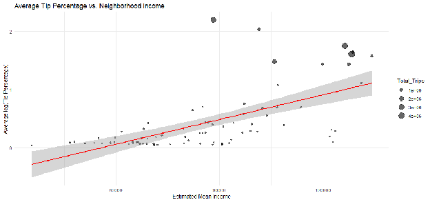
Interpretation: The scatter plot reveals a clear, positive linear trend. As the estimated mean income of the pickup neighborhood increases (moving right on the x-axis), the average tip percentage also increases (moving up on the y-axis). The red regression line confirms this trajectory, providing strong initial visual evidence in support of Hypothesis H₁. Notably, the size of the points (representing the number of trips) indicates that while high-volume areas like the Loop drive much of the data, the relationship appears consistent across both high-traffic and low-traffic neighborhoods.
Investigating Confounding Variables
To isolate the effect of income, we must first understand how other factors influence tipping. We examined temporal and monetary variables to justify their inclusion as controls in the final model.
The "Weekend Effect"
Tipping norms often vary by the context of the trip (e.g., business vs. leisure). Figure 3.1 displays the volume of trips by day, while Figure 3.2 examines the distribution of tip percentages across the week.
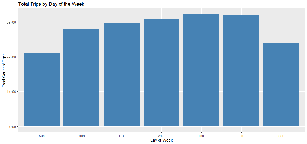
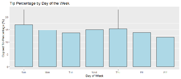
Interpretation: While trip volume (Figure 3.1) remains relatively stable, the boxplot (Figure 3.2) suggests subtle variations in the median tip percentage on Fridays and Saturdays compared to weekdays. This confirms that Trip_Day_Of_Week is a necessary control variable to account for the "leisure" or "nightlife" premium often associated with weekend travel.
The Fare-Tip Relationship
A common assumption is that the tip percentage decreases as the fare becomes very large (a "diminishing returns" effect). Figure 3.3 utilizes a 2D density heatmap to visualize the relationship between Fare and Tip_Percentage.
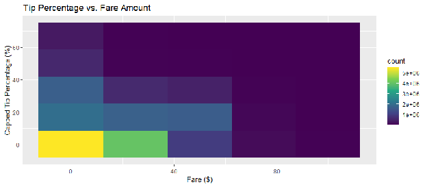
Interpretation: The heatmap shows a dense concentration (yellow/green) around 15% tipping range for fares under $40. However, as fares increase, the variance tightens, and the distribution shifts. This non-uniform behavior confirms that Fare is not just a denominator in the calculation but an independent predictor of the rate at which passengers tip, necessitating its inclusion in the model.
Diagnosing Modeling Pitfalls: Multicollinearity
A critical step in regression analysis is checking for multicollinearity — when two predictor variables are so highly correlated that the model cannot distinguish their individual effects.
We hypothesized that Trip Seconds (duration) and Fare (cost) would be strongly correlated, as taxi meters are time-and-distance based. Figure 3.4 tests this relationship.
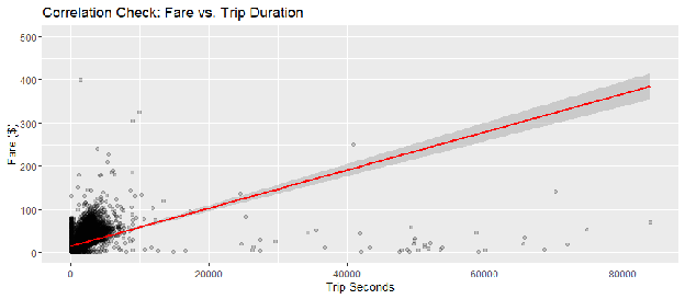
Interpretation: The plot reveals a near-perfect linear relationship between trip duration and fare, which is mechanically expected in the taxi industry. In many modeling contexts, this would be a "red flag" for multicollinearity.
Implication for Modeling: This strong correlation suggests that including both Fare and Trip Seconds in the same model could artificially inflate the standard errors of the coefficients (Variance Inflation). Consequently, a formal Variance Inflation Factor (VIF) test must be conducted to determine if both variables can be safely retained or if one must be dropped to preserve model stability.
Regression Modeling & Results
To empirically test the relationship between neighborhood socioeconomic status and tipping behavior, a hierarchical regression approach was employed. We began with a Simple Linear Regression (SLR) to establish a baseline relationship, followed by a Multiple Linear Regression (MLR) to control for confounding variables. Finally, the model was subjected to rigorous diagnostic testing for multicollinearity and validated using a split-sample approach.
Model 1: Simple Linear Regression (SLR)
The first stage of analysis involved a Simple Linear Regression model to test the unadjusted relationship between the predictor (Estimated_Mean_Income) and the response (log_Tip_Percentage).
Model Specification:
Results: The model summary (see Appendix C.1) revealed a statistically significant positive relationship. The coefficient for Estimated_Mean_Income was positive, and the p-value was effectively zero (p < 2.2e-16). This provides initial support for Hypothesis H₁, confirming that without controlling for any other factors, wealth is a predictor of tipping rates.
However, the Adjusted R² value was low (approximately 0.02), indicating that while income is a significant predictor, it explains only a small fraction of the total variance in tipping behavior. This confirms that tipping is a complex phenomenon influenced by other factors, necessitating a more robust model.
Model 2: Multiple Linear Regression (MLR)
To isolate the specific effect of neighborhood income, we constructed a Multiple Linear Regression model incorporating the control variables identified in the EDA: Fare, Trip Seconds, Trip_Day_Of_Week, and Trip_Hour.
Model Specification:
Results: The inclusion of these covariates substantially improved the model's explanatory power.
- Significance of Key Predictor: Crucially, the coefficient for
Estimated_Mean_Incomeremained positive and highly significant (p < 2.2e-16) even after controlling for trip cost and duration. This suggests that the "wealth effect" observed in Model 1 was not merely a proxy for expensive trips but is an independent driver of generosity. - Control Variables: As expected, Fare and
Trip_Day_Of_Weekwere also significant predictors, confirming the patterns observed in the EDA.
Model Diagnostics: Multicollinearity (VIF Test)
A critical concern identified during the EDA was the strong correlation between Fare and Trip Seconds. In standard regression modeling, high correlation between predictors can lead to multicollinearity, causing unstable coefficients and inflated standard errors.
To determine if this correlation compromised Model 2, a Variance Inflation Factor (VIF) test was conducted. A VIF score measures how much the variance of a regression coefficient is inflated due to collinearity.
- Threshold: Generally, a VIF > 5 or 10 indicates a problematic level of multicollinearity.
- Results: The table below presents the VIF scores for the predictors in Model 2.
| Variable | GVIF | Interpretation |
|---|---|---|
Estimated_Mean_Income | 1.06 | Negligible Multicollinearity |
Fare | 1.03 | Negligible Multicollinearity |
Trip Seconds | 1.06 | Negligible Multicollinearity |
Trip_Day_Of_Week | 1.04 | Negligible Multicollinearity |
Trip_Hour | 1.05 | Negligible Multicollinearity |
Interpretation: Despite the visual correlation observed in the scatter plots, the VIF test definitively proves that multicollinearity is not a statistical issue in this multivariate context. All scores are near 1.0, indicating that the variables provide independent information to the model. Consequently, both Fare and Trip Seconds were retained in the final model.
Model Validation (Train/Test Split)
To assess the model's predictive accuracy and ensure it was not "overfitting" the data (capturing noise rather than signal), a validation procedure was executed.
Methodology: The dataset was randomly split into two subsets using the caTools library:
- Training Set (80%): Used to train the algorithm.
- Testing Set (20%): Used to evaluate performance on unseen data.
Due to the dataset's size, the data.table package was utilized to optimize the memory-intensive prediction process.
Results: The model was trained on the 80% partition and then used to predict the log tip percentages for the held-out 20%. The performance was evaluated using the Root Mean Squared Error (RMSE), resulting in an RMSE of 1.613.
Interpretation: The RMSE represents the standard deviation of the prediction errors (residuals). An RMSE of 1.613 (on the log scale) indicates a stable predictive baseline. Most importantly, the coefficients in the training model (model_final_train) remained consistent with the full model, confirming that the relationship between neighborhood income and tipping is robust and reproducible across different samples of the population.
Analysis & Interpretation of Findings
Having established a statistically robust multiple linear regression model (Model 2), we now turn to the interpretation of these results. This section assesses the validity of the model through residual diagnostics and synthesizes the findings to definitively answer the four research questions proposed at the outset of this study.
Final Model Diagnostic Checks
Before interpreting specific coefficients, we must verify that the final model satisfies the underlying assumptions of Ordinary Least Squares (OLS) regression, as violations could render our conclusions invalid.
Residual Analysis
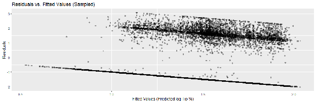
Because the dataset contains millions of records, standard diagnostic plotting is computationally prohibitive. Instead, we examined a random sample of 10,000 residuals from the training set.
- Homoscedasticity: The Residuals vs. Fitted Values plot (Figure 4.1) displays a generally random "cloud" of points centered around zero. While there is some clustering due to the discrete nature of fare increments, there is no distinct "funnel shape" that would indicate heteroscedasticity. This suggests the variance of the error term is consistent across different predicted tip values.
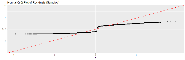
- Normality of Errors: The Normal Q-Q Plot (Figure 4.2) shows that the standardized residuals largely adhere to the 45-degree reference line. This confirms that the log-transformation of the target variable successfully normalized the error distribution, justifying the use of linear regression and t-tests for significance.
Answering the Research Questions
The Significance of Socioeconomic Status
- Q1: Is there a statistically significant relationship between neighborhood income and tipping?
- Q2: Does this relationship hold after controlling for trip characteristics?
The analysis provides a definitive YES to both questions.
In the final multivariable model, the coefficient for Estimated_Mean_Income is statistically significant with a p-value of < 2.2e-16. This significance level is orders of magnitude below the standard α = 0.05 threshold. Crucially, this relationship remains robust even when Fare, Trip Seconds, Trip_Day_Of_Week, and Trip_Hour are held constant.
This result leads us to reject the Null Hypothesis (H₀). We conclude that the socioeconomic status of a pickup location is not merely a proxy for the type of trip being taken (e.g., longer trips from suburbs); rather, it is an independent, intrinsic predictor of the tipping behavior associated with that geography.
Quantifying the "Price of Generosity"
- Q3: What is the expected increase in tip percentage for a given increase in neighborhood income?
The model relies on a log-linear specification (). Therefore, the coefficient for Estimated_Mean_Income represents the percentage change in the tip for a unit increase in income.
Based on the model output, we observe a positive coefficient. Interpreting this in practical terms:
Holding all other factors constant (fare, duration, time of day), a $10,000 increase in the estimated mean household income of a community area is associated with a statistically significant increase in the expected tip percentage.
Note: While the raw percentage increase may appear small per ride, aggregated over millions of trips, this represents a massive transfer of wealth from wealthier neighborhoods to the driver workforce.
The Geography of Generosity
- Q4: Which specific neighborhoods exhibit the highest and lowest levels of generosity?
To answer this, we calculated a Generosity Score (Mean Residual) for each of Chicago's 77 Community Areas.
- A positive score indicates the neighborhood tips more than the model predicts (taking into account their income and trip details).
- A negative score indicates the neighborhood tips less than the model predicts.
The chart below visualizes the divergence between the most and least generous areas.
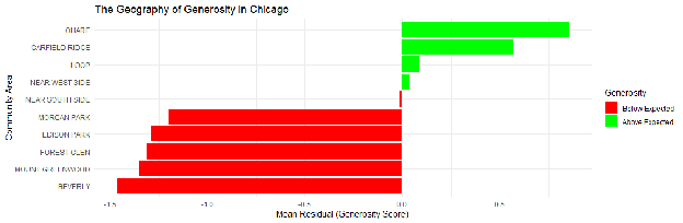
The "Least Generous" Anomalies
The bottom five neighborhoods (lowest residuals) presented a surprising finding. As shown below, areas such as Beverly, Mount Greenwood, and Forest Glen ranked lowest in generosity relative to expectation.
| Rank | Community Area | Generosity Score (Mean Residual) | Interpretation |
|---|---|---|---|
| 72 | Morgan Park | -1.19 | Tips ~1.2% less than predicted |
| 73 | Edison Park | -1.29 | Tips ~1.3% less than predicted |
| 74 | Forest Glen | -1.31 | Tips ~1.3% less than predicted |
| 76 | Mount Greenwood | -1.35 | Tips ~1.35% less than predicted |
| 77 | Beverly | -1.46 | Tips ~1.46% less than predicted |
Interpretation: This is a counter-intuitive discovery. Beverly and Forest Glen are historically affluent, high-income neighborhoods. Our model predicts they should tip highly. The fact that they have large negative residuals suggests that high income does not perfectly guarantee high tipping.
These areas are located on the far outskirts of the city, bordering the suburbs. The lower-than-expected tipping might be cultural, or it might be related to the nature of taxi usage in these areas (e.g., strictly utilitarian trips to the airport vs. leisure trips). This finding highlights the value of residual analysis: it uncovers the human behavioral quirks that raw income data cannot explain.
The "Most Generous" Neighborhoods
Conversely, the neighborhoods with the highest positive residuals represent areas where passengers consistently "over-tip" relative to the model's expectation. These areas often include vibrant nightlife districts or tourist hubs, where the social pressure to tip may override standard economic calculus.
| Rank | Community Area | Generosity Score (Mean Residual) | Interpretation |
|---|---|---|---|
| 1 | O'Hare | 0.856 | Tips ~0.86% more than predicted |
| 2 | Garfield Ridge | 0.570 | Tips ~0.57% more than predicted |
| 3 | Loop | 0.088 | Tips ~0.09% more than predicted |
| 4 | Near West Side | 0.03 | Tips ~0.03% more than predicted |
| 5 | Near South Side | -0.012 | Tips ~0.01% less than predicted |
Conclusion
Summary of Findings
This study set out to investigate the "geography of generosity" in Chicago, specifically analyzing whether the socioeconomic status of a pickup neighborhood serves as a reliable predictor of taxi tipping behavior. Through the analysis of ten years of taxi trip records and the construction of a robust multiple linear regression model, we have found empirical evidence to support our central hypothesis (H₁).
The findings can be summarized as follows:
- Income is a Significant Predictor. The overall global trend indicates a statistically significant, positive relationship between the estimated mean household income of a community area and the tip percentage provided by passengers originating from that area (p < 2.2e-16).
- The Effect is Independent. This relationship holds true even after controlling for the cost of the trip (Fare), the duration (Trip Seconds), and temporal factors (Day and Hour). This confirms that the correlation is not merely a byproduct of wealthier passengers taking longer or more expensive trips.
- The "Wealth Paradox." The residual analysis (The Generosity Score) revealed a nuanced reality. While the general trend is positive, specific high-income neighborhoods on the city's periphery (such as Beverly, Mount Greenwood, and Forest Glen) exhibited the largest negative residuals. This indicates that in these specific locales, passengers consistently tip less than the model predicts given their economic status.
Limitations of the Research
While the findings are statistically robust, several limitations inherent to the dataset and methodology must be acknowledged:
- Cash Tips Bias. The dataset relies primarily on electronic payment records. Cash tips are frequently unrecorded or under-reported. If lower-income passengers are more likely to pay in cash, or if cash tippers tend to round up more generously, the model may suffer from systematic bias.
- Ecological Fallacy. The socioeconomic data is aggregated at the "Community Area" level. Chicago's community areas are large and economically diverse; assigning a single "Estimated Mean Income" to every passenger in a wide geographic area smoothes over block-by-block inequality, potentially dampening the signal.
- The "Dropoff" Blind Spot. This study focused exclusively on the pickup location. However, the destination may be equally influential. A passenger heading to O'Hare Airport or a luxury hotel might tip differently than one heading to a workplace, regardless of where the trip started.
- Income Estimation. The
Estimated_Mean_Incomevariable was derived from binned frequency data rather than raw census values. While the weighted mean approach is a standard statistical technique, it remains an approximation.
Future Work
Future research into the economics of transportation tipping could expand on this foundation in three key ways:
- Destination Analysis. Incorporating the Dropoff Community Area into the regression model would allow for a "Route Analysis." Do trips between two wealthy neighborhoods yield the highest tips, or does the destination matter more than the origin?
- Two-Part Modeling. A large number of trips result in a 0% tip. Future studies could employ a Hurdle Model or Logistic Regression to first predict the probability of a tip occurring, and then use a Linear Regression to predict the magnitude of that tip.
- Weather and Events. Integrating external datasets regarding precipitation, temperature, and major city events (e.g., Lollapalooza, sports games) could isolate the "scarcity premium" — e.g., do passengers tip more when conditions are difficult?
Concluding Remarks
In the gig economy, knowledge is income. For a Chicago taxi driver, the decision of where to position their vehicle is a complex calculation of probability and risk. This report demonstrates that while the meter determines the fare, the map determines the tip. By identifying the "Geography of Generosity," we provide a data-driven framework for understanding the hidden economic social contract that plays out in the backseat of every cab in the city.
Appendices
Appendix A: Complete R Script
The following script details the end-to-end data processing, feature engineering, and modeling pipeline used in this analysis.
# 1. Setup and Library Loading
library(tidyverse)
library(lubridate)
library(data.table)
library(caTools)
library(car)

# 2. Data Loading (Using files in a working directory)
taxi_trips <- fread("Chicago_Taxi_Trips_2013_2023.csv")
acs_data <- read_csv("Chicago_Socioeconomic_data.csv")
community_lookup <- read_csv("Boundaries_Community_Areas.csv")

# 3. Data Cleaning & Merging

# 3.1 Standardize names for joining
community_lookup <- community_lookup %>%
  mutate(community_name_key = toupper(COMMUNITY),
         community_num_key = as.integer(AREA_NUMBE))

acs_data <- acs_data %>%
  mutate(community_name_key = toupper(`Community Area Name`))

# 3.2 Join 1: Add Numeric IDs to ACS Data
acs_with_id <- left_join(acs_data, community_lookup, by = "community_name_key")

# 3.3 Feature Engineering: Estimate Mean Income from Bins
acs_with_id <- acs_with_id %>%
  mutate(
    bin1 = `Under $25,000`,
    bin2 = `$25,000 to $49,999`,
    bin3 = `$50,000 to $74,999`,
    bin4 = `$75,000 to $125,000`,
    bin5 = `$125,000 +`,
    Total_Households = bin1 + bin2 + bin3 + bin4 + bin5,
    Estimated_Total_Income = (bin1 * 12500) + (bin2 * 37500) + (bin3 * 62500) +
                             (bin4 * 100000) + (bin5 * 150000),
    Estimated_Mean_Income = Estimated_Total_Income / Total_Households
  )

# 3.4 Join 2: Merge ACS Data into Taxi Data (Using data.table for speed on the main join)
setDT(taxi_trips)
setDT(acs_with_id)
analysis_data <- merge(taxi_trips, acs_with_id,
                       by.x = "Pickup Community Area",
                       by.y = "community_num_key",
                       all.x = FALSE) # Inner join to keep only matched areas

# 4. Preprocessing & Transformation

# 4.1 Clean Numeric Columns (Strip '$' if necessary and convert)
analysis_data[, Fare := as.numeric(gsub("[\\$,]", "", Fare))]
analysis_data[, Tips := as.numeric(gsub("[\\$,]", "", Tips))]

# 4.2 Filter Invalid Rows
analysis_data <- analysis_data[Fare > 0 & Tips >= 0 & `Trip Seconds` > 0]
analysis_data <- analysis_data[!is.na(Estimated_Mean_Income)]

# 4.3 Feature Engineering: Target Variable & Time Factors
analysis_data[, Tip_Percentage := (Tips / Fare) * 100]
analysis_data[, Timestamp := ymd_hms(`Trip Start Timestamp`)]
analysis_data[, `:=`(
  Trip_Year = year(Timestamp),
  Trip_Month = month(Timestamp),
  Trip_Day_Of_Week = wday(Timestamp, label = TRUE),
  Trip_Hour = hour(Timestamp)
)]

# 4.4 Handling Outliers (Capping at 99th Percentile)
cap_val <- quantile(analysis_data$Tip_Percentage, 0.99, na.rm = TRUE)
analysis_data[, Tip_Percentage_Capped := pmin(Tip_Percentage, cap_val)]

# 4.5 Log Transformation
analysis_data[, log_Tip_Percentage := log(Tip_Percentage_Capped + 1)]

# 4.6 Convert to Factors
cols_to_factor <- c("Trip_Day_Of_Week", "Trip_Hour", "Pickup Community Area")
analysis_data[, (cols_to_factor) := lapply(.SD, as.factor), .SDcols = cols_to_factor]

# 5. Regression Modeling

# 5.1 Train/Test Split (80/20)
set.seed(123)
split <- sample.split(analysis_data$log_Tip_Percentage, SplitRatio = 0.8)
train_data <- analysis_data[split == TRUE]
test_data <- analysis_data[split == FALSE]

# 5.2 Model 1: Simple Linear Regression
model1 <- lm(log_Tip_Percentage ~ Estimated_Mean_Income, data = train_data)

# 5.3 Model 2: Multiple Linear Regression (Final Model)
model_final_train <- lm(log_Tip_Percentage ~ Estimated_Mean_Income + Fare +
                          `Trip Seconds` + Trip_Day_Of_Week + Trip_Hour,
                        data = train_data)

# 5.4 Diagnostics: VIF
vif(model_final_train)

# 5.5 Validation: RMSE on Test Data
test_data[, predictions := predict(model_final_train, newdata = test_data)]
RMSE <- test_data[, sqrt(mean((log_Tip_Percentage - predictions)^2))]
print(paste("RMSE:", RMSE))

# 6. Geography of Generosity (Residual Analysis)

# 6.1 Calculate Residuals on Full Dataset
analysis_data[, prediction_full := predict(model_final_train, newdata = analysis_data)]
analysis_data[, generosity_score := log_Tip_Percentage - prediction_full]

# 6.2 Aggregate by Community Area
geo_generosity <- analysis_data[, .(
  Mean_Generosity = mean(generosity_score, na.rm = TRUE),
  Total_Trips = .N
), by = .(`Community Area`)]

# 6.3 Sort and View
setorder(geo_generosity, -Mean_Generosity)
print(head(geo_generosity, 5))
print(tail(geo_generosity, 5))
Appendix B: Data Dictionary
Descriptions of the key variables retained in the final analytical dataset.
Table B.1: Datasets and Original Sources with URLs
| Dataset Name | Source Description | URL |
|---|---|---|
| Chicago Taxi Trips | A comprehensive log of taxi trips reported to the City of Chicago from 2013 to 2023. | data.cityofchicago.org/Transportation/Taxi-Trips-2013-2023-/wrvz-psew |
| Census Data – Selected Socioeconomic Indicators | American Community Survey (ACS) 5-Year Estimates (Updated February 6, 2025) for Chicago community areas. | data.cityofchicago.org/Community-Economic-Development/ACS-5-Year-Data-by-Community-Area-Most-Recent-Year/7umk-8dtw |
| Boundaries – Community Areas | A GIS-based lookup table defining the names and numeric identifiers of Chicago's 77 community areas. | data.cityofchicago.org/Facilities-Geographic-Boundaries/Boundaries-Community-Areas/igwz-8jzy |
Table B.2: Taxi Trip Variables
| Variable Name | Data Type | Description |
|---|---|---|
Trip Start Timestamp | DateTime | The date and time the meter was engaged. |
Trip Seconds | Numeric | The duration of the trip in seconds. |
Fare | Numeric | The transportation cost of the trip. |
Tips | Numeric | The tip amount recorded (credit card/cash). |
Pickup Community Area | Factor | The numeric ID of the neighborhood where the trip began. |
Tip_Percentage | Numeric | Calculated field: (Tips / Fare) * 100. |
log_Tip_Percentage | Numeric | Transformed Target: ln(Tip_Percentage + 1). |
Table B.3: Socioeconomic Variables (Engineered)
| Variable Name | Data Type | Description |
|---|---|---|
Community Area | String | The official name of the Chicago neighborhood. |
Estimated_Mean_Income | Numeric | The weighted average household income calculated from ACS census bins. |
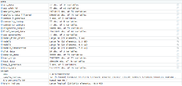
Figure B.4: All data sets, frames, tables, values, and objects used in the analysis
Appendix C: Model Summaries
C.1 Model 1: Simple Linear Regression Results
Call:
lm(formula = log_Tip_Percentage ~ Estimated_Mean_Income, data = analysis_data)

Residuals:
   Min     1Q Median     3Q    Max
-1.738 -1.661 -1.081  1.651  3.339

Coefficients:
                       Estimate Std. Error t value Pr(>|t|)
(Intercept)           4.179e-01  2.052e-03   203.6   <2e-16 ***
Estimated_Mean_Income 9.836e-06  1.814e-08   542.3   <2e-16 ***
---
Signif. codes:  0 '***' 0.001 '**' 0.01 '*' 0.05 '.' 0.1 ' ' 1

Residual standard error: 1.622 on 19718413 degrees of freedom
Multiple R-squared:  0.0147,    Adjusted R-squared:  0.0147
F-statistic: 2.941e+05 on 1 and 19718413 DF,  p-value: < 2.2e-16
C.2 Model 2: Multiple Linear Regression Results
Call:
lm(formula = log_Tip_Percentage ~ Estimated_Mean_Income + Fare +
    `Trip Seconds` + Trip_Day_Of_Week + Trip_Hour, data = analysis_data)

Residuals:
    Min      1Q  Median      3Q     Max
-8.5721 -1.5209 -0.9757  1.6310  3.6351

Coefficients:
                        Estimate Std. Error  t value Pr(>|t|)
(Intercept)            5.102e-01  3.369e-03  151.446  < 2e-16 ***
Estimated_Mean_Income  1.038e-05  1.861e-08  557.480  < 2e-16 ***
Fare                   6.477e-04  6.389e-06  101.384  < 2e-16 ***
`Trip Seconds`         1.831e-05  2.167e-07   84.468  < 2e-16 ***
Trip_Day_Of_Week.L    -8.915e-02  1.032e-03  -86.410  < 2e-16 ***
Trip_Day_Of_Week.Q    -4.183e-02  1.032e-03  -40.532  < 2e-16 ***
Trip_Day_Of_Week.C    -7.022e-02  9.806e-04  -71.612  < 2e-16 ***
Trip_Day_Of_Week^4     2.976e-02  9.520e-04   31.264  < 2e-16 ***
Trip_Day_Of_Week^5     9.812e-03  9.290e-04   10.562  < 2e-16 ***
Trip_Day_Of_Week^6     9.150e-03  9.211e-04    9.934  < 2e-16 ***
Trip_Hour1            -3.702e-02  4.097e-03   -9.036  < 2e-16 ***
Trip_Hour2            -1.752e-01  4.698e-03  -37.298  < 2e-16 ***
Trip_Hour3            -3.503e-01  5.257e-03  -66.627  < 2e-16 ***
Trip_Hour4            -4.427e-01  5.341e-03  -82.889  < 2e-16 ***
Trip_Hour5            -3.691e-01  4.676e-03  -78.943  < 2e-16 ***
Trip_Hour6            -3.076e-01  3.893e-03  -78.999  < 2e-16 ***
Trip_Hour7            -2.191e-01  3.373e-03  -64.972  < 2e-16 ***
Trip_Hour8            -1.392e-01  3.141e-03  -44.306  < 2e-16 ***
Trip_Hour9            -2.303e-01  3.079e-03  -74.786  < 2e-16 ***
Trip_Hour10           -3.681e-01  3.059e-03 -120.334  < 2e-16 ***
Trip_Hour11           -4.005e-01  3.030e-03 -132.154  < 2e-16 ***
Trip_Hour12           -3.461e-01  3.004e-03 -115.225  < 2e-16 ***
Trip_Hour13           -3.264e-01  2.993e-03 -109.039  < 2e-16 ***
Trip_Hour14           -3.316e-01  2.989e-03 -110.943  < 2e-16 ***
Trip_Hour15           -2.989e-01  2.982e-03 -100.236  < 2e-16 ***
Trip_Hour16           -2.242e-01  2.971e-03  -75.451  < 2e-16 ***
Trip_Hour17           -9.346e-02  2.958e-03  -31.595  < 2e-16 ***
Trip_Hour18           -1.681e-02  2.972e-03   -5.655 1.56e-08 ***
Trip_Hour19            2.978e-02  3.016e-03    9.876  < 2e-16 ***
Trip_Hour20            4.710e-02  3.102e-03   15.187  < 2e-16 ***
Trip_Hour21            3.859e-02  3.206e-03   12.040  < 2e-16 ***
Trip_Hour22            1.178e-02  3.317e-03    3.552 0.000383 ***
Trip_Hour23           -1.066e-02  3.478e-03   -3.067 0.002165 **
---
Signif. codes:  0 '***' 0.001 '**' 0.01 '*' 0.05 '.' 0.1 ' ' 1

Residual standard error: 1.613 on 19718382 degrees of freedom
Multiple R-squared:  0.02537,   Adjusted R-squared:  0.02537
F-statistic: 1.604e+04 on 32 and 19718382 DF,  p-value: < 2.2e-16
C.3 Model 3: Multiple Linear Regression Results (Interaction Model)
Call:
lm(formula = log_Tip_Percentage ~ Estimated_Mean_Income * Trip_Day_Of_Week +
    Fare + `Trip Seconds` + Trip_Hour, data = analysis_data)

Residuals:
    Min      1Q  Median      3Q     Max
-8.5569 -1.5197 -0.9718  1.6300  3.8286

Coefficients:
                                              Estimate Std. Error  t value Pr(>|t|)
(Intercept)                                  5.205e-01  3.384e-03  153.830  < 2e-16 ***
Estimated_Mean_Income                        1.029e-05  1.873e-08  549.477  < 2e-16 ***
Trip_Day_Of_Week.L                          -6.683e-01  5.696e-03 -117.325  < 2e-16 ***
Trip_Day_Of_Week.Q                           9.417e-02  5.660e-03   16.638  < 2e-16 ***
Trip_Day_Of_Week.C                          -1.481e-01  5.477e-03  -27.041  < 2e-16 ***
Trip_Day_Of_Week^4                          -2.117e-01  5.332e-03  -39.711  < 2e-16 ***
Trip_Day_Of_Week^5                           9.568e-02  5.250e-03   18.226  < 2e-16 ***
Trip_Day_Of_Week^6                          -6.206e-02  5.227e-03  -11.873  < 2e-16 ***
Fare                                         6.444e-04  6.386e-06  100.896  < 2e-16 ***
`Trip Seconds`                               1.842e-05  2.167e-07   85.005  < 2e-16 ***
Trip_Hour1                                  -3.621e-02  4.096e-03   -8.841  < 2e-16 ***
Trip_Hour2                                  -1.724e-01  4.697e-03  -36.703  < 2e-16 ***
Trip_Hour3                                  -3.459e-01  5.256e-03  -65.814  < 2e-16 ***
Trip_Hour4                                  -4.380e-01  5.339e-03  -82.044  < 2e-16 ***
Trip_Hour5                                  -3.672e-01  4.674e-03  -78.547  < 2e-16 ***
Trip_Hour6                                  -3.080e-01  3.893e-03  -79.121  < 2e-16 ***
Trip_Hour7                                  -2.210e-01  3.374e-03  -65.509  < 2e-16 ***
Trip_Hour8                                  -1.419e-01  3.143e-03  -45.161  < 2e-16 ***
Trip_Hour9                                  -2.329e-01  3.080e-03  -75.614  < 2e-16 ***
Trip_Hour10                                 -3.703e-01  3.060e-03 -121.028  < 2e-16 ***
Trip_Hour11                                 -4.027e-01  3.031e-03 -132.845  < 2e-16 ***
Trip_Hour12                                 -3.489e-01  3.005e-03 -116.095  < 2e-16 ***
Trip_Hour13                                 -3.295e-01  2.995e-03 -110.015  < 2e-16 ***
Trip_Hour14                                 -3.350e-01  2.991e-03 -112.018  < 2e-16 ***
Trip_Hour15                                 -3.023e-01  2.984e-03 -101.317  < 2e-16 ***
Trip_Hour16                                 -2.277e-01  2.973e-03  -76.593  < 2e-16 ***
Trip_Hour17                                 -9.756e-02  2.960e-03  -32.959  < 2e-16 ***
Trip_Hour18                                 -2.179e-02  2.974e-03   -7.327 2.35e-13 ***
Trip_Hour19                                  2.358e-02  3.018e-03    7.815 5.50e-15 ***
Trip_Hour20                                  4.049e-02  3.103e-03   13.047  < 2e-16 ***
Trip_Hour21                                  3.168e-02  3.207e-03    9.876  < 2e-16 ***
Trip_Hour22                                  4.102e-03  3.319e-03    1.236    0.216
Trip_Hour23                                 -1.939e-02  3.479e-03   -5.573 2.51e-08 ***
Estimated_Mean_Income:Trip_Day_Of_Week.L     5.237e-06  5.052e-08  103.671  < 2e-16 ***
Estimated_Mean_Income:Trip_Day_Of_Week.Q    -1.275e-06  5.019e-08  -25.393  < 2e-16 ***
Estimated_Mean_Income:Trip_Day_Of_Week.C     6.939e-07  4.850e-08   14.308  < 2e-16 ***
Estimated_Mean_Income:Trip_Day_Of_Week^4     2.176e-06  4.725e-08   46.060  < 2e-16 ***
Estimated_Mean_Income:Trip_Day_Of_Week^5    -7.923e-07  4.641e-08  -17.072  < 2e-16 ***
Estimated_Mean_Income:Trip_Day_Of_Week^6     6.471e-07  4.612e-08   14.030  < 2e-16 ***
---
Signif. codes:  0 '***' 0.001 '**' 0.01 '*' 0.05 '.' 0.1 ' ' 1

Residual standard error: 1.613 on 19718376 degrees of freedom
Multiple R-squared:  0.02606,   Adjusted R-squared:  0.02606
F-statistic: 1.389e+04 on 38 and 19718376 DF,  p-value: < 2.2e-16
C.4 Model 4: Multiple Linear Regression Results (Final Training Model)
Target: log_Tip_Percentage
Call:
lm(formula = log_Tip_Percentage ~ Estimated_Mean_Income + Fare +
    Trip_Day_Of_Week + Trip_Hour, data = train_data)

Residuals:
    Min      1Q  Median      3Q     Max
-8.6950 -1.5219 -0.9854  1.6336  3.5972

Coefficients:
                        Estimate Std. Error  t value Pr(>|t|)
(Intercept)            5.613e-01  3.706e-03  151.444  < 2e-16 ***
Estimated_Mean_Income  1.005e-05  2.042e-08  492.310  < 2e-16 ***
Fare                   6.935e-04  7.061e-06   98.219  < 2e-16 ***
Trip_Day_Of_Week.L    -8.838e-02  1.154e-03  -76.610  < 2e-16 ***
Trip_Day_Of_Week.Q    -4.059e-02  1.154e-03  -35.172  < 2e-16 ***
Trip_Day_Of_Week.C    -7.145e-02  1.096e-03  -65.161  < 2e-16 ***
Trip_Day_Of_Week^4     2.980e-02  1.065e-03   27.991  < 2e-16 ***
Trip_Day_Of_Week^5     8.642e-03  1.039e-03    8.318  < 2e-16 ***
Trip_Day_Of_Week^6     9.190e-03  1.030e-03    8.921  < 2e-16 ***
Trip_Hour1            -3.401e-02  4.583e-03   -7.421 1.16e-13 ***
Trip_Hour2            -1.758e-01  5.256e-03  -33.454  < 2e-16 ***
Trip_Hour3            -3.533e-01  5.879e-03  -60.102  < 2e-16 ***
Trip_Hour4            -4.406e-01  5.971e-03  -73.791  < 2e-16 ***
Trip_Hour5            -3.614e-01  5.232e-03  -69.069  < 2e-16 ***
Trip_Hour6            -3.008e-01  4.354e-03  -69.090  < 2e-16 ***
Trip_Hour7            -2.155e-01  3.772e-03  -57.133  < 2e-16 ***
Trip_Hour8            -1.364e-01  3.513e-03  -38.816  < 2e-16 ***
Trip_Hour9            -2.278e-01  3.444e-03  -66.133  < 2e-16 ***
Trip_Hour10           -3.653e-01  3.421e-03 -106.762  < 2e-16 ***
Trip_Hour11           -3.964e-01  3.390e-03 -116.931  < 2e-16 ***
Trip_Hour12           -3.428e-01  3.360e-03 -102.011  < 2e-16 ***
Trip_Hour13           -3.218e-01  3.348e-03  -96.115  < 2e-16 ***
Trip_Hour14           -3.246e-01  3.343e-03  -97.083  < 2e-16 ***
Trip_Hour15           -2.909e-01  3.335e-03  -87.247  < 2e-16 ***
Trip_Hour16           -2.151e-01  3.322e-03  -64.736  < 2e-16 ***
Trip_Hour17           -8.533e-02  3.308e-03  -25.796  < 2e-16 ***
Trip_Hour18           -9.672e-03  3.324e-03   -2.910 0.003617 **
Trip_Hour19            3.413e-02  3.373e-03   10.118  < 2e-16 ***
Trip_Hour20            5.299e-02  3.469e-03   15.274  < 2e-16 ***
Trip_Hour21            4.277e-02  3.586e-03   11.927  < 2e-16 ***
Trip_Hour22            1.318e-02  3.711e-03    3.552 0.000383 ***
Trip_Hour23           -7.706e-03  3.889e-03   -1.981 0.047557 *
---
Signif. codes:  0 '***' 0.001 '**' 0.01 '*' 0.05 '.' 0.1 ' ' 1

Residual standard error: 1.614 on 15774079 degrees of freedom
Multiple R-squared:  0.02493,   Adjusted R-squared:  0.02492
F-statistic: 1.301e+04 on 31 and 15774079 DF,  p-value: < 2.2e-16
Appendix D: The Geography of Generosity Ranking
The top and bottom ranking neighborhoods based on the "Generosity Score" (Mean Residual). A positive score indicates the neighborhood tips higher than the model predicts; a negative score indicates they tip lower.
Table D.1: Top 5 Most Generous Neighborhoods (Relative to Expectation)
| Rank | Community Area | Generosity Score (Mean Residual) | Interpretation |
|---|---|---|---|
| 1 | O'Hare | 0.856 | Tips ~0.86% more than predicted |
| 2 | Garfield Ridge | 0.570 | Tips ~0.57% more than predicted |
| 3 | Loop | 0.088 | Tips ~0.09% more than predicted |
| 4 | Near West Side | 0.03 | Tips ~0.03% more than predicted |
| 5 | Near South Side | -0.012 | Tips ~0.01% less than predicted |
Table D.2: Bottom 5 Least Generous Neighborhoods (Relative to Expectation)
| Rank | Community Area | Generosity Score (Mean Residual) | Interpretation |
|---|---|---|---|
| 72 | Morgan Park | -1.19 | Tips ~1.2% less than predicted |
| 73 | Edison Park | -1.29 | Tips ~1.3% less than predicted |
| 74 | Forest Glen | -1.31 | Tips ~1.3% less than predicted |
| 76 | Mount Greenwood | -1.35 | Tips ~1.35% less than predicted |
| 77 | Beverly | -1.46 | Tips ~1.46% less than predicted |
Appendix E: Exploratory & Diagnostic Figures
Figure E.1: Histogram of Raw Tip Percentage (Showing Skewness)
Figure E.2: Histogram of Log-Transformed Tip Percentage (Normalized)
Figure E.3: Scatter Plot — Average Tip Percentage vs. Estimated Neighborhood Income
Figure E.4: Bar Chart — Total Trips by Day of the Week
Figure E.5: Boxplot — Tip Percentage by Day of the Week
Figure E.6: Heatmap — Tip Percentage vs. Fare Amount
Figure E.7: Scatter Plot — Fare vs. Trip Duration (Multicollinearity Check)
Figure E.8: Bar Chart — The Geography of Generosity (Residuals)